Static Characteristics Of Instruments|EEE Made Easy

static characteristics of instruments:The attributes collectively known as the static characteristics of instruments and are given in the datasheet for a particular instrument.

The 11 main Static characteristics of instruments are given below;

Accuracy and inaccuracy (measurement uncertainty)
Precision/repeatability/reproducibility
Tolerance
Range or span
Linearity
Sensitivity of measurement
Threshold
Resolution
Sensitivity to disturbance
Hysteresis effects
Dead space

Download & Install EEE Made Easy App

Static characteristics of instruments

What do you mean by the Static characteristics of instruments?

static characteristics of instruments:The attributes collectively known as the static characteristics of instruments and are given in the datasheet for a particular instrument.

It is important to note that the values quoted for instrument characteristics in such a data sheet only apply when the instrument is used under specified standard calibration conditions.

Due allowance must be made for variations in the characteristics when the instrument is used in other conditions.

You can visit EEE Made Easy Bookstore HERE

What are the Static characteristics of instruments?

1. Accuracy and inaccuracy (measurement uncertainty)

The accuracy of an instrument is a measure of how close the output reading of the instrument is to the correct value.

In practice, it is more usual to quote the inaccuracy figure rather than the accuracy figure for an instrument.

Inaccuracy is the extent to which reading might be wrong and is often quoted as a percentage of the full-scale (f.s.) reading of an instrument.

If, for example, a pressure gauge of range 0–10 bar has a quoted inaccuracy of +/- 1.0% f.s. (+/- 1% of full-scale reading), then the maximum error to be expected in any reading is 0.1 bar.

This means that when the instrument is reading 1.0 bar, the possible error is 10% of this value.

For this reason, it is an important system design rule that instruments are chosen such that their range is appropriate to the spread of values being measured, in order that the best possible accuracy is maintained in instrument readings.

Thus, if we were measuring pressures with expected values between 0 and 1 bar, we would not use an instrument with a range of 0–10 bar.

The term measurement uncertainty is frequently used in place of inaccuracy.

2. Precision/repeatability/reproducibility

Precision is a term that describes an instrument’s degree of freedom from random errors.

If a large number of readings are taken of the same quantity by a high precision instrument, then the spread of readings will be very small.

Precision is often, though incorrectly, confused with accuracy.

High precision does not imply anything about measurement accuracy.

A high precision instrument may have low accuracy.

Low accuracy measurements from a high precision instrument are normally caused by a bias in the measurements, which is removable by recalibration.

What are repeatability and reproducibility?

The terms repeatability and reproducibility mean approximately the same but are applied in different contexts.

Repeatability

Repeatability describes the closeness of output readings when the same input is applied repetitively over a short period of time, with the same measurement conditions, same instrument and observer, same location and same conditions of use maintained throughout.

Reproducibility

Reproducibility describes the closeness of output readings for the same input when there are changes in the method of measurement, observer, measuring instrument, location, conditions of use and time of measurement.

Both terms thus describe the spread of output readings for the same input.

This spread is referred to as repeatability if the measurement conditions are constant and as reproducibility, if the measurement conditions vary.

The degree of repeatability or reproducibility in measurements from an instrument is an alternative way of expressing its precision.

3. Tolerance

Tolerance is a term that is closely related to accuracy and defines the maximum error that is to be expected in some value.

Whilst it is not, strictly speaking, a static characteristic of measuring instruments, it is mentioned here because the accuracy of some instruments is sometimes quoted as a tolerance figure.

When used correctly, tolerance describes the maximum deviation of a manufactured component from some specified value.

For instance, electric circuit components such as resistors have

tolerances of perhaps 5%.

One resistor is chosen at random from a batch having a nominal

value 1000W and tolerance 5% might have an actual value anywhere between 950W and 1050 W.

4. Range or span

The range or span of an instrument defines the minimum and maximum values of the quantity that the instrument is designed to measure.

5. Linearity

It is normally desirable that the output reading of an instrument is linearly proportional to the quantity being measured.

In a plot of the typical output readings of an instrument when a sequence of input quantities are applied to it, the normal procedure is to draw a good fit straight line through the points.

The non-linearity is then defined as the maximum deviation of any of the output readings marked points from this straight line.

Non-linearity is usually expressed as a percentage of full-scale reading.

6. Sensitivity of measurement

The sensitivity of measurement is a measure of the change in instrument output that occurs when the quantity being measured changes by a given amount.

Thus, sensitivity is the ratio of scale deflection to the value of measurand producing deflection.

The sensitivity of measurement is, therefore, the slope of the straight line drawn based on the values.

If, for example, a pressure of 2 bar produces a deflection of 10 degrees in a pressure transducer, the sensitivity of the instrument is 5 degrees/bar

(assuming that the deflection is zero with zero pressure applied).

7. Threshold

If the input to an instrument is gradually increased from zero, the input will have to reach a certain minimum level before the change in the instrument output reading is of a large enough magnitude to be detectable.

This minimum level of input is known as the threshold of the instrument.

Manufacturers vary in the way that they specify a threshold for instruments.

Some quote absolute values, whereas others quote threshold as a percentage of full-scale readings.

As an illustration, a car speedometer typically has a threshold of about 15 km/h. This means that, if the vehicle starts from rest and accelerates, no output reading is observed on the speedometer until the speed reaches 15 km/h.

8 Resolution

When an instrument is showing a particular output reading, there is a lower limit on the magnitude of the change in the input measured quantity that produces an observable change in the instrument output.

Like threshold, the resolution is sometimes specified as an absolute value and sometimes as a percentage of f.s. deflection.

One of the major factors influencing the resolution of an instrument is how finely its output scale is divided into subdivisions.

Using a car speedometer as an example again, this has subdivisions of typically 20 km/h.

This means that when the needle is between the scale markings, we cannot estimate speed more accurately than to the nearest 5 km/h. This figure of 5 km/h thus represents the resolution of the instrument.

9. Sensitivity to disturbance

All calibrations and specifications of an instrument are only valid under controlled conditions of temperature, pressure etc.

These standard ambient conditions are usually defined in the instrument specification.

As variations occur in the ambient temperature etc., certain static instrument characteristics change, and the sensitivity to disturbance

is a measure of the magnitude of this change.

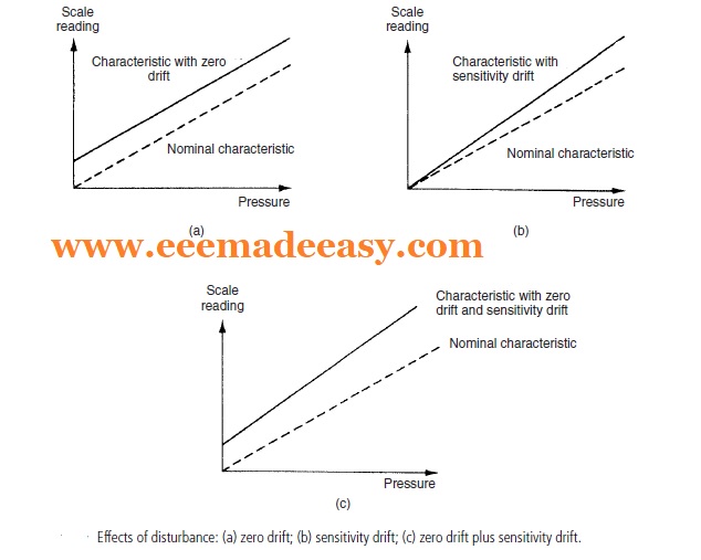
Such environmental changes affect instruments in two main ways, known as zero drift and sensitivity drift.

what is Zero drift?

Zero drift is sometimes known by the alternative term, bias.

Zero drift or bias describes the effect where the zero reading of an instrument is modified by a change in ambient conditions.

This causes a constant error that exists over the full range of measurement of the instrument.

The mechanical form of a bathroom scale is a common example of an instrument that is prone to bias.

It is quite usual to find that there is a reading of perhaps 1 kg with no one stood on the scale.

If someone of known weight 70 kg were to get on the scale, the reading would be 71 kg, and if someone of known weight 100 kg were to get on the scale, the reading would be 101 kg.

How can we remove the Zero drift of Instruments?

Zero drift is normally removable by calibration.

In the case of the bathroom scale just described, a thumbwheel is usually provided that can be turned until the reading is zero with the scales unloaded, thus removing the bias.

Zero drift is also commonly found in instruments like voltmeters that are affected by ambient temperature changes.

Typical units by which such zero drift is measured are volts/°C.

This is often called the zero drift coefficient related to temperature changes.

If the characteristic of an instrument is sensitive to several environmental parameters, then it will have several zero drift coefficients, one for each environmental parameter.

What is Sensitivity drift?

Sensitivity drift (also known as scale factor drift) defines the amount by which an instrument’s sensitivity of measurement varies as ambient conditions change.

It is quantified by sensitivity drift coefficients that define how much drift there is for a unit change in each environmental parameter that the instrument characteristics are sensitive to.

Many components within an instrument are affected by environmental fluctuations, such as temperature changes: for instance, the modulus of elasticity of spring is temperature-dependent.

Sensitivity drift is measured in units of the form (angular degree/bar)/°C.

If an instrument suffers both zero drift and sensitivity drift at the same time, then the typical modification of the output characteristic is shown in Figure (c)

10. Hysteresis effects

hysteresis characteristics of instruments

The above fig. illustrates the output characteristic of an instrument that exhibits hysteresis.

If the input measured quantity to the instrument is steadily increased from a negative value, the output reading varies in the manner shown in curve (a).

If the input variable is then steadily decreased, the output varies in the manner shown in curve (b).

The non-coincidence between these loading and unloading curves is known as hysteresis.

Two quantities are defined, maximum input hysteresis and maximum output hysteresis, as shown in Figure above.

These are normally expressed as a percentage of the full-scale

input or output reading respectively.

11. Dead space

Dead space is defined as the range of different input values over which there is no change in output value.

Any instrument that exhibits hysteresis also displays dead space, as marked on Figure explaining hysteresis characteristics.

Some instruments that do not suffer from any significant hysteresis can still exhibit a dead space in their output characteristics, however.

Backlash in gears is a typical cause of dead space and results in the sort of instrument output characteristic shown in Figure below.

instrument characteristics with deadspace

Backlash is commonly experienced in gearsets used to convert between translational and rotational motion (which is a common technique used to measure translational velocity).

You can check the previous posts also.

Here there are some books for studying Measurements and Instrumentation and some Electrical & Electronics Text Books